The road to Fathom is long and hard.

Throughout my time at Fathom, I’ve been lucky enough to get to know everyone in the group at a personal level. Whether that’s talking about indie video games with Katherine after lunch, watching Hot Frosty and making pizzas with Ellory, looking at cool fish with Kyle, or any number of other activities, it’s been really special to learn from everyone both professionally and personally. However, only one of these has turned into a somewhat consistent out-of-work commitment: running to the shop with Mark.

Mark, for those of you less familiar, is a sensational developer and, shall we say, a strikingly unique musician. In his own estimation, Mark says: “I know what I like, but I’m also acutely aware of the fact that I might be the only person in the world who likes it.” I feel that Mark’s approach to data is driven by his empathy and interest in philosophy; hearing his descriptions of data make it come to life, make it feel like a beast one is trying to wrangle or a curious plant one has just discovered in the midst of a forest. Mark lends a tangible sense of purpose to each piece of software he builds. For all this unity of intention that Mark embodies, however, he is not single-faceted. Beyond his many other talents, everything about him screams ‘runner:’ his long limbs, his limber gait, and his persistence and consistency as a programmer.

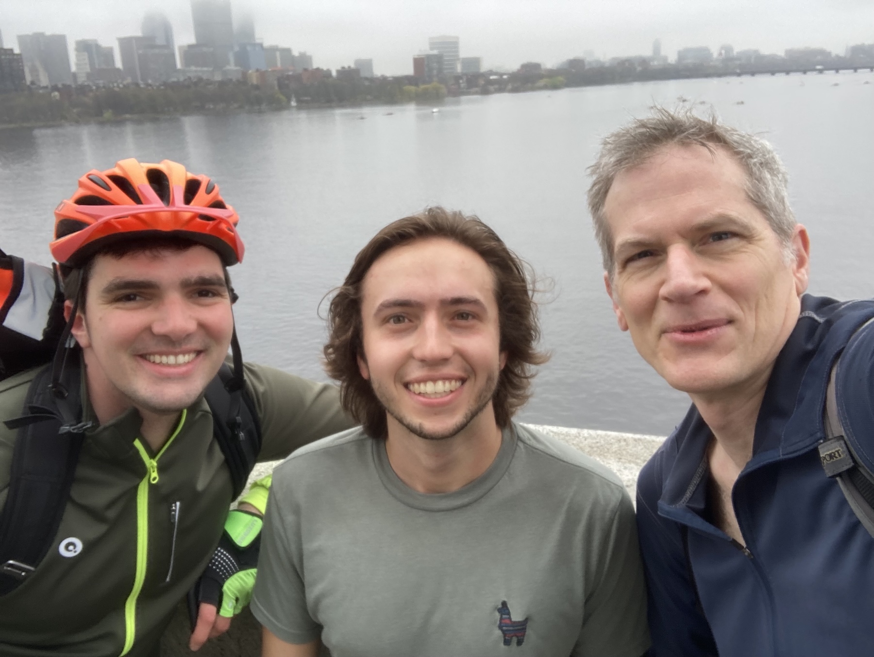
Well, as a runner myself, this gave Mark and I just one more thing to talk about. After almost 8 months of working at Fathom, we finally made the spur-of-the-moment decision to run to work together. Paul accompanied us on his trusty bike, acting as a guidepost of sorts, as we toiled away through the empty streets of Cambridge.

This might sound all fun and games, but it wasn’t without difficulty. I live in the rapidly gentrifying neighborhood of Lower Allston, whereas Mark hails from the far-off land of Arlington. In addition, I’m usually a morning person, but my roommates are not; waking up at 6:00 or 6:30am is a challenge in and of itself. Still, we managed to meet up at Harvard Square, not too far off of Mark’s usual route into Boston. And Paul the Biker’s fleeting but ever-returning presence taught us by metaphor that any suffering we felt in the moment was transient, and would soon be replaced by the comforting joy of visualizing data.

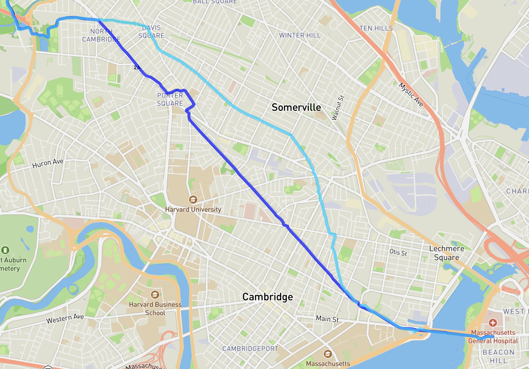
We went on six more runs over the following months, varying our starting point and pace depending on the day. Generally, we took one of two routes through Somerville, seen in the bluish lines below. Well, I’m sure you’re wondering: did we improve? Ha. I’m surprised you even had to ask. Let’s take a look at our progress so far.

What are the important pieces of the puzzle in this data story? Well, for Mark at least, the total distance of the run is always the same, so we’re not too concerned with that. Let’s start by checking pace (minutes per mile) to see if that improves over time.

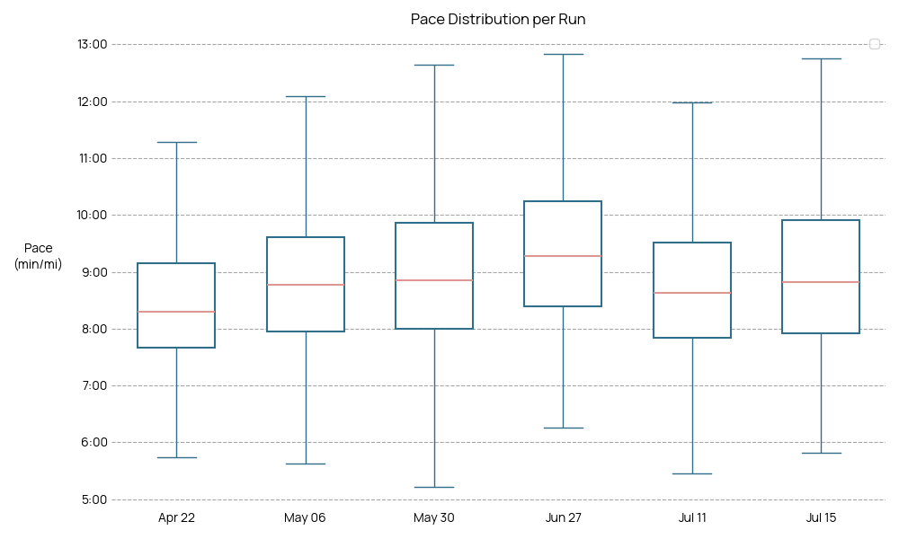
These are boxplots of Mark and my pace for each run. As you can see, our pace varies significantly; elevation changes, stop lights, and a million other things are actively trying to prevent us from running in the city. The bar within the box is our median pace (usually around 9:30 minutes per mile), and the box itself spans the middle 50% of the data.

While the boxes have slightly different sizes and positions, there’s really not a big noticeable difference across runs. But, how can we tell if there is a statistically significant difference? Well, we can do that with a one-way analysis of variance test (one-way ANOVA). In our case, it will tell us if at least one of the runs is statistically different from any of the others. If there was a sharp increase or decrease in our performance in any run, this will tell us. And it turns out…

No difference!

Each run is not statistically separable from the other runs by pace alone. The variation we see visually could just be due to chance (p=0.460). Does that mean Mark and I didn’t get any better at running? Of course not. Let’s think about what else could be going on here.

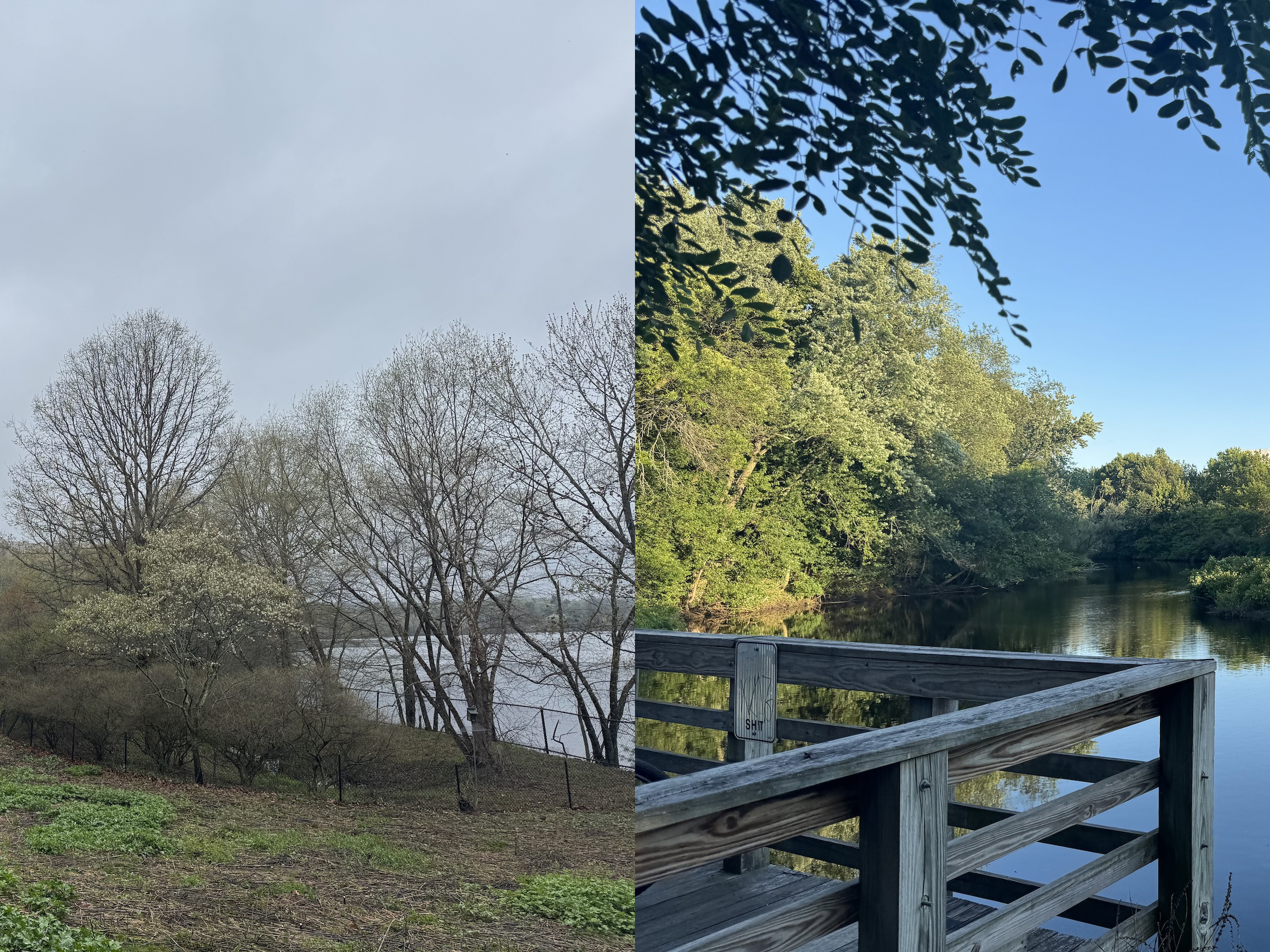
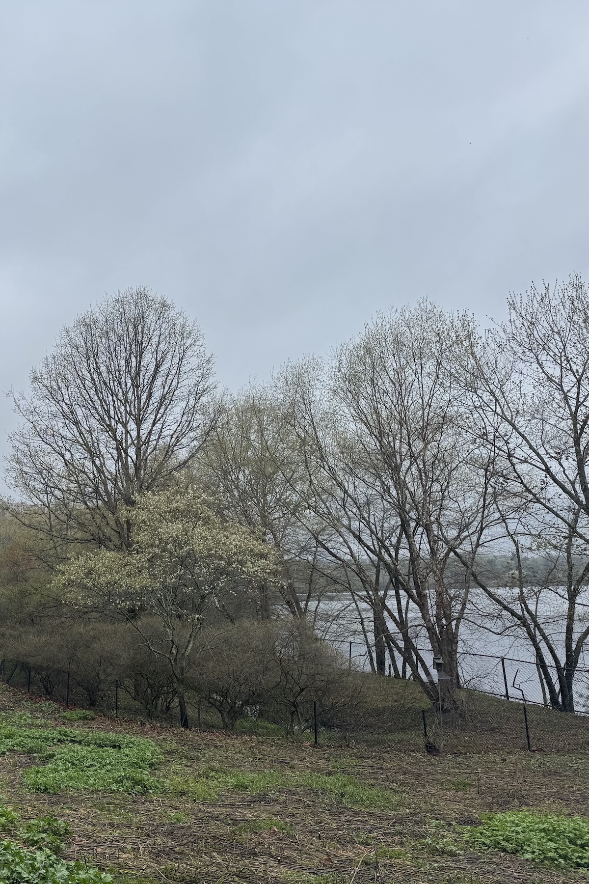
Take a look at the date for each run. We started this journey in late April and ran throughout July. In Cambridge and Boston, the weather completely changes from the spring to the summer! From the relative cold of late April eventually comes the humid heat of June. Heat probably makes it harder to run, but the question is: how much harder?

In any long-form physical activity, wet-bulb temperature is a key environmental metric. If you cover the bulb of a thermometer with a wet cloth, water will evaporate and cool the bulb, thereby lowering the temperature. However, if the air is more humid, water has more difficulty evaporating, preventing the bulb from cooling. This is the same with sweat, which we humans use quite a bit to maintain our body temperature. A wet-bulb temperature of around 95˚F is considered the upper limit for human survival. The experience of 90˚F in the dry deserts of California is not as physically intense as 90˚F humid air along the coastline of Massachusetts.

In case you’re interested in the details, this is how we calculate wet bulb temperature from drybulb temperature and relative humidity:

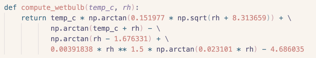
Specifically, we’ll use a modified version called Wet Bulb Global Temperature (WBGT), which is often cited in medical literature. Below is an approximate formula for calculating that:

And now, we can see the average wet bulb global temperature for each of our runs:

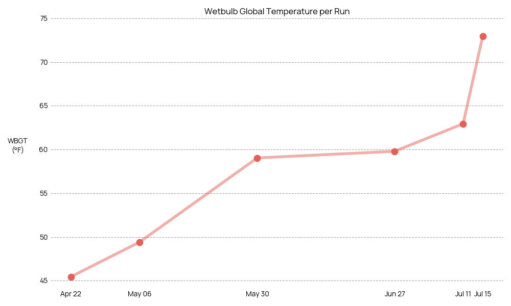
According to Konstantinos Mantzios et al. 2021 in “Effects of Weather Parameters on Endurance Running Performance: Discipline-specific Analysis of 1258 Races,” each 1.8˚F of WBGT outside of an optimal range (45.5˚F – 59˚F) leads to a performance decline of 0.3%-0.4%. Note that related literature cites similar ranges, and uses this effect to estimate expected race times in alternate weather conditions. We can apply this to our running paces to get a new set of distributions and compare the differences. Was our actual pace better than we expected given the hotter temperatures?

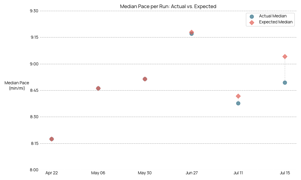
Especially on those hotter runs, you can really see the difference! The red diamonds are the values we expect given our temperature model, assuming our overall performance was the same as when we started. Both with time and with increasing temperature, you can see our overall performance increases, as our actual median pace becomes visibly faster than the expected pace.

Using a paired t-test to compare the actual vs. expected paces, we do find a highly significant difference (p<0.0005), albeit with a relatively small effect size (Cohen’s d=-0.455).

Maybe it was just a refusal to go slower no matter the weather, or maybe our fitness really did improve. Either way, we do see significantly higher performance levels on our summer runs compared to spring. Mark, we did it!

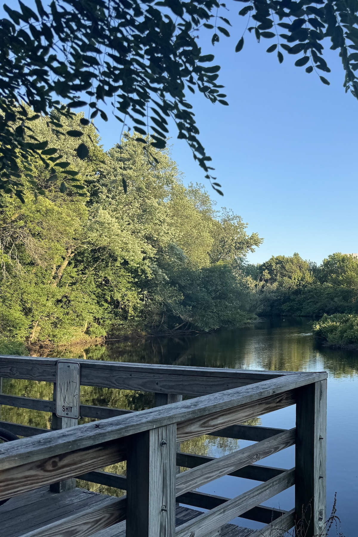
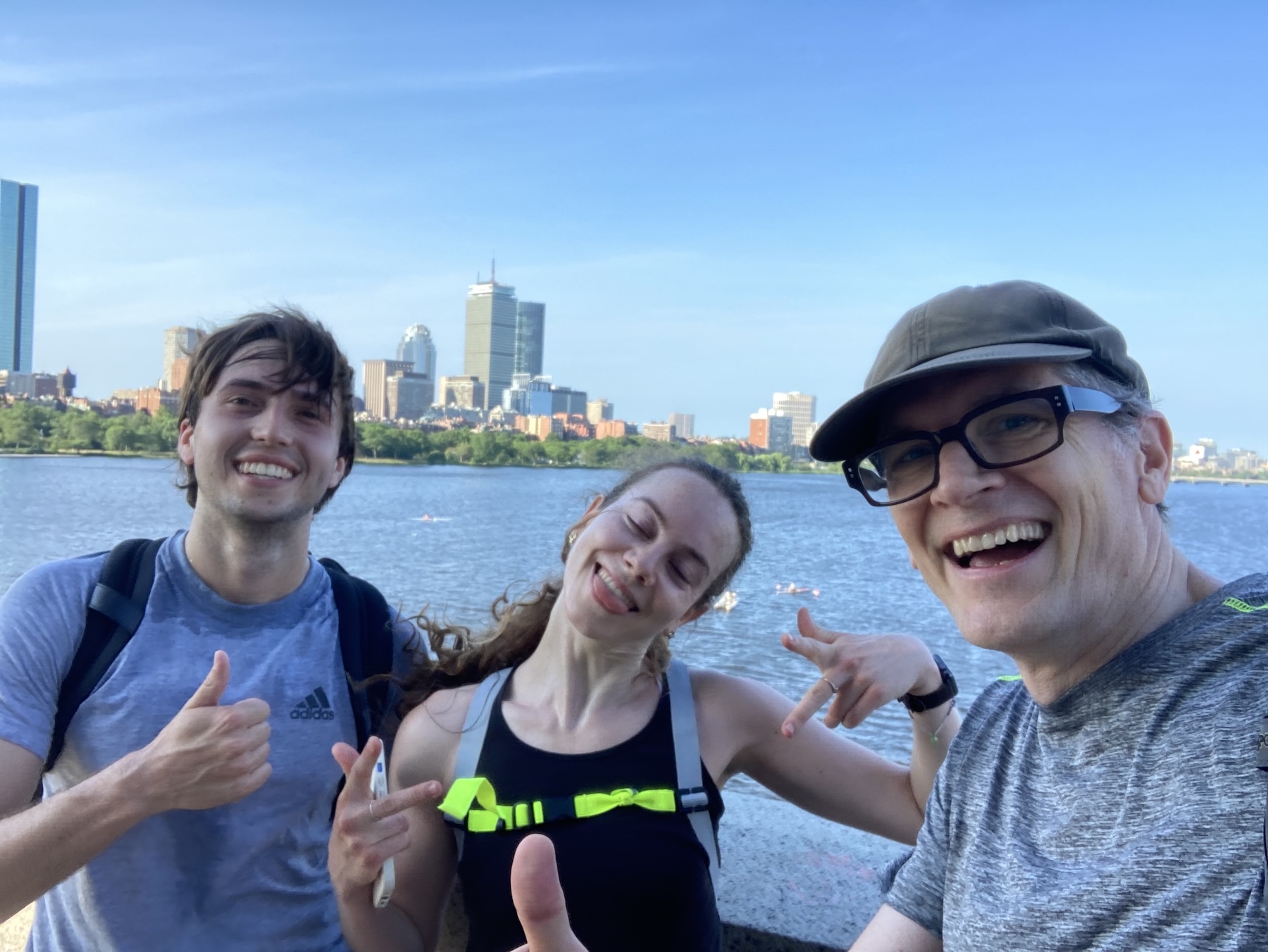
While the data is fun to explore, it only captures so much. When I look back on these runs, I’ll be thinking about the conversations we had, the sights we saw, and moments like Paul joining us for our first run and Libby joining us for our last.

I couldn’t have asked for a better way to learn from Mark and to get to know him as a person. And, this is just one example of the moments and stories that are core to everyone’s experience at Fathom. Look forward to hearing about more Fathomite adventures around Boston!